

‘This blog assumes some familiarity with traditional machine learning, neural networks, probability & statistics and linear algebra.‘
In the last blog, we introduced you to Artificial Intelligence, now we are going to discuss the details of computer vision.
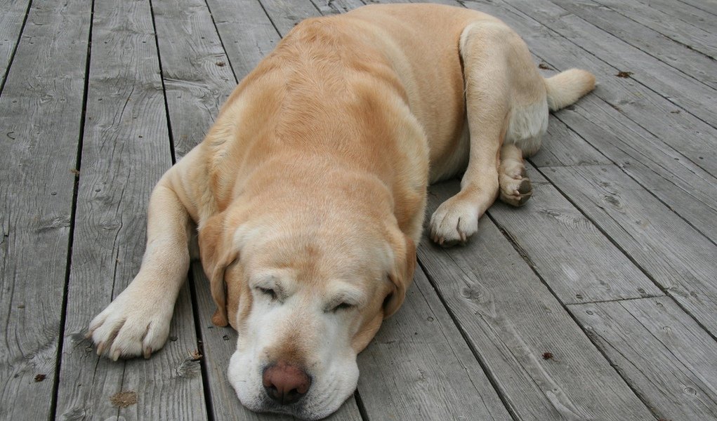
Look at this picture of a dog and a cat.
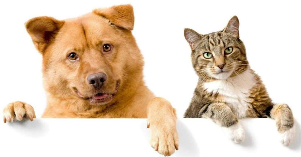
How we humans easily distinguish between a dog and a cat? It did not take even seconds for our brain to distinguish between them. But let us think for a second about how we actually do that? The answer is we have seen (or similar) them before and we are trained well in distinguishing between a cat and a dog, but we are looking for a more basic answer- how will you teach a child who have not seen animals before to distinguish between a cat and a dog? Think before seeing the answer.
So, you will tell their salient features which makes them differentiable. Maybe their ears, eyes, mouth, all the things that make them differentiable from each other. These features will help the child’s brain to differentiate between them.
This process is similar for a machine as well. We need to extract features from images of cat and dog to differentiate between them and train a model on the basis of that. But still we don’t understand that how we actually extract salient features from images?
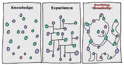
Another thing is we need a really large corpus of images of cats and dogs to make a model because a model trained on a small set of images may lead to overfitting ( read the intro to A.I. with the example of shoes ).
We need to tackle few problems first-
- If computer understands only 0 and 1 i.e. binaries how is it going to understand images ?
- In computers, alphabets are represented by ASCII value and numbers are encoded in binaries. So, we need someway to represent an image into numbers. I guess we all know how is that possible.
The basic building block of image is a PIXEL which is a number. So one problem is solved to display an image as an 2-D array of numbers (pixels).
- How to extract features from the image?
- This is the most important question to ask, how do we extract features from images. It can be done in few ways ( sorted in increasing popularity ) –
1. Traditional Machine Learning – It is the oldest and the most tedious method of extracting features. In this we extract features manually and use machine learning algorithms like RandomForestClassifier (tree based models), SVM ( non-tree based models) to train our model. Extracted features are stored using columns for every image and preparing a CSV file out of it. Also, in the target column the number of classes are equal to number of object we want to classify.
This is not a good approach for computer vision, this process is very tedious and we can’t manually extract all features. The accuracy from these type of modelling is often not good. (~50%).
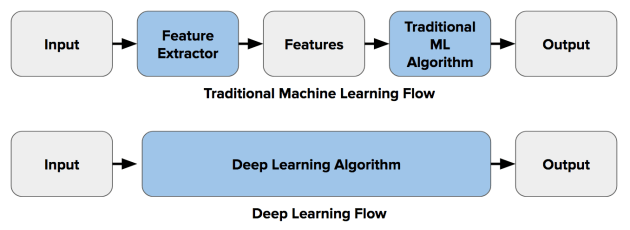
2. Dense Neural Network – With the introduction of deep learning field in Machine learning, the task of computer vision (specially) became much easy and successful. The use of dense neural network was very successful for computer vision ( I won’t go in the deep of dense neural network as this is the prerequisite of this blog ). The main difference between traditional methods and DNN was that the task of feature extraction became automated i.e. now we don’t need to extract features manually. The results were quite amazing at beginning. But it faced two problem one solvable and the other was problematic.
First problem was compute power. DNN requires a hell lot of compute power to work . Initially it use to take hours if not days to solve a simple classification computer vision problem using DNN. This problem was solved with the introduction of more powerful compute engines like GPU, TPU. The another main problem it faced was huge which initially does not seemed to be a problem. The training accuracy after DNN was amazing ( ~ 90+%) but the test accuracy was very bad. The problem was when we feed the 2D array of pixels to a DNN ( we have to flatten the array to convert it to 1D because dnn takes 1D array as input) it finds pattern for the same type of picture only. Rather than finding features for the object, it finds pattern for the whole image. So, when in the test data, any image with slightly different configuration comes, the models fails miserably to work. For ex. – If the model is trained using these types of images of a dog –
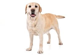
And in the test data it finds an image of the dog in different position or configuration like
It fails miserably. The model in the above case finds non-linear relation/ pattern in the whole image rather than finding features of the dog. So, some further work was needed to resolve this big issue . The solution came as CNN .
3. Convolution Neural Network (CNN) – This is the state of art choice for computer Vision these days. Rather than feeding the images directly to the DNN, we apply a kind of filter to all the images. These filter helps to extract useful information and features from the images, removing all the noises from it and then applying the DNN network to it. These special type of filters is known as Convolution.
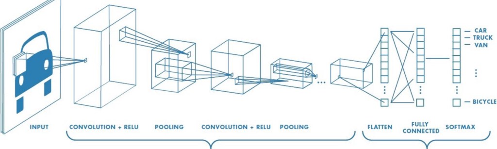
These convolution filter are nothing but n*n matrix ( where n is odd ) which is multiplied to every pixel of the image and a new array is made out of it, which represents useful features.
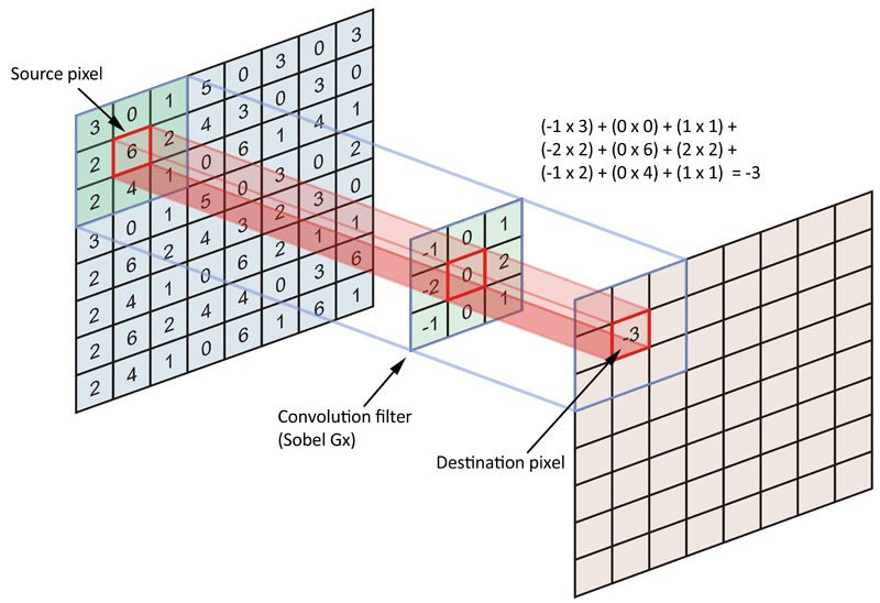
There are many types of convolution filters used for different purposes and we use a lot of them while this process. The problem occurs when the number of images increases manifolds because as we apply many filter to a single image producing a filtered image for every filter, there are many many images produced and it requires very much computational power and hours to train. The solution is a very useful algorithm named MaxPooling. MaxPooling is an approach of taking the maximum value from a m*m table and removing all other values. So, after applying convolution every time we should use MaxPooling to make the image small without losing important features. After this we need to convert the formed 2D array to 1D array and feed it to DNN. The results of CNN are quite amazing and state of art.
Now, we know the theory of computer vision but before moving towards coding part, let us discuss another important issue – Overfitting.
Overfitting happens when we achieve great accuracy for train data but very bad accuracy for test data. The reason for overfitting is less amount of data available for training or the available data is not a well distributed. For ex.- If for classifying between horse and zebra we have every image of horse sitting and zebra standing in train set, the model will predict zebra even for standing horse and horse even for a sitting zebra in test.
This problem is huge and there are different number of ways to eradicate or reduce it –
- Data Augmentation – It is the process of increasing the train data by manipulating the train images, this process tackles both the problems of overfitting. The manipulation can be by rotating the images at different angles, zooming the image, flipping the image and so on.
2.Transfer Learning – This is more recent and more successful technique. Many researchers and experts in DL field have made state of art models using millions of images and the best compute power in world to train their models. These models contains thousands of layers and state of art accuracy. If we have a small train data available to us, we can use weights from these so called pre-trained models to train our local model. We don’t need to train their whole model, we can just take weights of their DNN and use it for our model to increase manyfolds.
( There are more technique like use of Dropout in DNN to solve the problem of overfitting, but we won’t go in details of that )
Now, enough of theory. Let us learn to code. We will be using Tensorflow which is a framework developed by Google for Deep learning problems. It uses great abstraction and make the task of deep learning very easy to learn and code. Further, we will be using high-level API of Tensorflow named Keras. For the basics of it, you can go to website of http://www.tensorflow.org(and look for tutorials.
We will be showing examples for CNN using tensorflow. You can code on Google Colab which is a web-based notebook which has the same interface as Jupyter notebook provided by Google in which you can use GPU, TPU from your local machine.
First of all, all of this makes sense but the most basic that we get is how we are going to import images to our notebook to work on it. First, the train images in your local machine ( in case of using colab, it should be first uploaded to google drive ) should be stored in their respective label folder which in turn should be stored in another folder name train. For ex. If you want to make a classifier for horse and human images. You should have all horse images in a folder name horse and all human images in a folder named human. These folder horse and human should be under directory named Train. Then use this code –
| import keras_preprocessing | |
| from keras_preprocessing.image import ImageDataGenerator | |
| TRAINING_DIR = "/tmp/rps/" | |
| training_datagen = ImageDataGenerator( | |
| rescale = 1./255, | |
| ) | |
| train_generator = training_datagen.flow_from_directory( | |
| TRAINING_DIR, | |
| target_size=(150,150), | |
| class_mode=‘binary’, | |
| batch_size=126 | |
| ) |
Here ‘TRAINING_DIR’ is the directory address of train, ‘rescale’ is use for rescaling all the pixels because neural nets are scale variant, ‘target_size’ is the size we want of every image and ‘class_mode’ is the classification if it is binary class problem then use binary else categorical.
Now, the task of preparing the CNN model-
| model = tf.keras.models.Sequential([ | |
| # Note the input shape is the desired size of the image 150x150 with 3 bytes color | |
| # This is the first convolution | |
| tf.keras.layers.Conv2D(64, (3,3), activation='relu', input_shape=(150, 150, 3)), | |
| tf.keras.layers.MaxPooling2D(2, 2), | |
| # The second convolution | |
| tf.keras.layers.Conv2D(64, (3,3), activation='relu'), | |
| tf.keras.layers.MaxPooling2D(2,2), | |
| # The third convolution | |
| tf.keras.layers.Conv2D(128, (3,3), activation='relu'), | |
| tf.keras.layers.MaxPooling2D(2,2), | |
| # The fourth convolution | |
| tf.keras.layers.Conv2D(128, (3,3), activation='relu'), | |
| tf.keras.layers.MaxPooling2D(2,2), | |
| # Flatten the results to feed into a DNN | |
| tf.keras.layers.Flatten(), | |
| tf.keras.layers.Dropout(0.5), | |
| # 512 neuron hidden layer | |
| tf.keras.layers.Dense(512, activation='relu'), | |
| tf.keras.layers.Dense(2, activation='softmax') | |
| ]) | |
| model.compile(loss = 'categorical_crossentropy', optimizer='rmsprop', metrics=['accuracy']) | |
| history = model.fit(train_generator, epochs=25, steps_per_epoch=20, validation_data = validation_generator, verbose = 1, validation_steps=3) |
Here we have used 4 layers of CNN layers. The arguments in CNN layers are (the number of filters, size of filters, activation) whereas always remember that the size of first layer should be equal to the shape of the array (input_shape).
Also, we used categorical crossentropy as loss function here , for a binary class we could also use sigmoid activation in last layer instead of softmax and binary_crossentropy loss instead of categorical_crossentropy.
There are a lot of choices of optimisers like Adam, rmsprop, gradient descent. We can choose best using parameter hyper tuning.
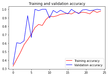
Also, the task of visualisation of train accuracy and test accuracy can be done using –
| import matplotlib.pyplot as plt | |
| acc = history.history['accuracy'] | |
| val_acc = history.history['val_accuracy'] | |
| loss = history.history['loss'] | |
| val_loss = history.history['val_loss'] | |
| epochs = range(len(acc)) | |
| plt.plot(epochs, acc, 'r', label='Training accuracy') | |
| plt.plot(epochs, val_acc, 'b', label='Validation accuracy') | |
| plt.title('Training and validation accuracy') | |
| plt.legend(loc=0) | |
| plt.figure() | |
| plt.show() |
Finally, if we achieve overfitting. We can use data augmentation and Transfer learning very easily in Tensorflow.
Data Augmentation
| train_datagen = ImageDataGenerator(rescale = 1./255., | |
| rotation_range = 40, | |
| width_shift_range = 0.2, | |
| height_shift_range = 0.2, | |
| shear_range = 0.2, | |
| zoom_range = 0.2, | |
| horizontal_flip = True) |
Here every image is changed into 6 images with different configurations like rotation, zoom, height_shift, width_shift, flip. Here float value shows range out of 1.
Also, the process of Transfer Learning is very easy in Tensorflow. But we have to keep in mind that there are many pre-trained models available and we should choose pre-trained model according to our task.
For ex. We will be using Inception V3 model for training our model of classifying cats and dogs.
| from tensorflow.keras.applications.inception_v3 import InceptionV3 | |
| local_weights_file = '/tmp/inception_v3_weights_tf_dim_ordering_tf_kernels_notop.h5' | |
| pre_trained_model = InceptionV3(input_shape = (150, 150, 3), | |
| include_top = False, | |
| weights = None) | |
| pre_trained_model.load_weights(local_weights_file) | |
| for layer in pre_trained_model.layers: | |
| layer.trainable = False | |
| # pre_trained_model.summary() | |
| last_layer = pre_trained_model.get_layer('mixed7') | |
| print('last layer output shape: ', last_layer.output_shape) | |
| last_output = last_layer.output |
A pre-trained model comprises of many layers and we can take weight from any layer, although it is advised not to take weights from both extremes. Also, we have to make pre-trained model freezes so that it does not get retrained on our data.
Here, we took weights of a layer named ‘mixed7’ from the model.
How to use it? Well, pretty similar to above CNN model but with a slight modification
| from tensorflow.keras.optimizers import RMSprop | |
| From tensorflow.keras import Model | |
| From tensorflow.keras.models import layers | |
| # Flatten the output layer to 1 dimension | |
| x = layers.Flatten()(last_output) | |
| # Add a fully connected layer with 1,024 hidden units and ReLU activation | |
| x = layers.Dense(1024, activation='relu')(x) | |
| # Add a dropout rate of 0.2 | |
| x = layers.Dropout(0.2)(x) | |
| # Add a final sigmoid layer for classification | |
| x = layers.Dense (1, activation='sigmoid')(x) | |
| model = Model( pre_trained_model.input, x) | |
| model.compile(optimizer = RMSprop(lr=0.0001), | |
| loss = 'binary_crossentropy', | |
| metrics = ['accuracy']) |
If you read the code properly you will find it very similar to above (I’ll leave it to you)
After this, The best task will be to start your own project or maybe try competing on Kagglehttp://www.kaggle.com using these method. This blog will give you a overview of CNN and its code with tensorflow. If you face any difficulty feel free to ping me.
Ciao.
Cogitare Et Credere
